728x90
728x90
1. Attention 기반 ASR 모델
Attention 기반 자동 음성 인식(ASR)은 기존의 CTC 방식과 달리 입력 음성 특징과 출력 테스트 간의 정렬(alignment)을 명시적으로 학습할 수 있는 장점을 가진 방식이다. 이 방식은 특히 Encoder-Decoder 구조와 결합하여 문장 단위의 인식, 불규칙한 정렬, 다양한 언어 구조에 대응할 수 있다.
📌 구조
[입력 음성] -> Encoder -> Attention -> Decoder -> [문자 시퀀스]
- Encoder: 음성 신호(MFCC, Mel Spectrogram 등)를 입력받아 시퀀스 형태의 고차원 벡터로 변환
- Attention: 인코더의 출력 중 어디에 집중할지를 계산
- Decoder: 한 글자씩 생성하면서 Attention 가중치를 사용
📌 Attention을 이용한 Word 기반 ASR
# 1. 데이터 로드 및 Mel-Spectrogram 추출
file_paths = sorted(glob("recordings/*.wav"))

def extract_mel_features(file_list, sr=16000, n_mels=80):
    X, y = [], []
    for path in file_list:
        label = os.path.basename(path)[0]
        waveform, _ = librosa.load(path, sr=sr)
        mel = librosa.feature.melspectrogram(y=waveform, sr=sr, n_mels=n_mels)  # 입력 waveform을 Mel-Spectrogram으로 변환
        mel_db = librosa.power_to_db(mel, ref=np.max)
        mel_db = librosa.util.normalize(mel_db).T  # 정규화 + 전치
        X.append(mel_db)
        y.append(label)
    return X, y

X, y = extract_mel_features(file_paths)
label_encoder = LabelEncoder()
y_encoded = label_encoder.fit_transform(y)

# 시퀀스 길이 패딩
maxlen = max([x.shape[0] for x in X])
X_pad = tf.keras.preprocessing.sequence.pad_sequences(X, maxlen=maxlen, padding='post', dtype='float32')

# 학습/검증 데이터 분할
X_train, X_val, y_train, y_val = train_test_split(X_pad, y_encoded, test_size=0.2, random_state=42)
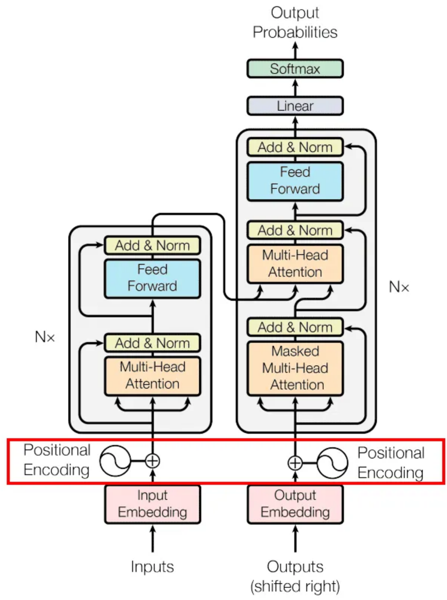
※ Positional Encoding 추가
- 시계열 데이터의 프레임 순서 정보를 추가함
- Transformer는 순서를 직접 알 수 없기 때문에 위치 정보를 더해야 함
- 각 시간 위치 tt에 해당하는 고유한 벡터를 생성하여 입메딩에 더함
- 모델이 각 프레임이 문장 앞인지 뒤인지 구별 가능하게 됨
# 2. Positional Encoding 레이어 정의
class PositionalEncoding(tf.keras.layers.Layer):
    def call(self, x):
        seq_len = tf.shape(x)[1]
        d_model = tf.shape(x)[2]

        pos = tf.cast(tf.range(seq_len)[:, tf.newaxis], tf.float32)     # [T, 1]
        i = tf.cast(tf.range(d_model)[tf.newaxis, :], tf.float32)       # [1, D]

        angle_rates = 1 / tf.pow(10000., (2 * (i // 2)) / tf.cast(d_model, tf.float32))
        angle_rads = pos * angle_rates

        angle_rads = tf.where(i % 2 == 0, tf.cos(angle_rads), tf.sin(angle_rads))  # [T, D]
        return x + angle_rads[tf.newaxis, :, :]  # [1, T, D] broadcasting
# 3. 모델 정의 함수 (Conv1D + Attention + Dense 구조)
def build_model(input_shape, num_classes):
# 입력층: 입력 shape은 (time_steps, 80), 여기서 80은 Mel feature 개수
inputs = tf.keras.Input(shape=input_shape) # [T, 80]
# 1단계: Conv1D로 지역적인 시간 패턴 추출 (예: 자음, 모음의 경계)
# 필터 수 128개, 커널 크기 5, ReLU 활성화
x = tf.keras.layers.Conv1D(
filters=128,
kernel_size=5,
padding='same',
activation='relu'
)(inputs) # 출력 shape: [T, 128]
# 2단계: Batch Normalization으로 학습 안정화 및 수렴 속도 향상
x = tf.keras.layers.BatchNormalization()(x) # 출력 shape: [T, 128]
# 3단계: Dense 레이어를 통해 차원 조정 (다음 단계에서 position encoding 적용하기 위함)
# Conv1D의 출력 128차원을 그대로 유지하되, 이 레이어가 학습 가능한 임베딩 역할을 수행
x = tf.keras.layers.Dense(128)(x) # 출력 shape: [T, 128]
# 4단계: Positional Encoding 추가 (Transformer 구조에서 필수)
# 입력 시퀀스에 순서 정보를 더해줌 (위치 정보가 없으면 self-attention은 순서를 인식 못함)
x = PositionalEncoding()(x) # 출력 shape: [T, 128]
# 5단계: Multi-Head Self-Attention
# 각 프레임이 전체 프레임을 참고하여 문맥 정보를 반영하도록 함
# num_heads=2 → 독립된 주의집중 기법을 2개 동시에 수행
x = tf.keras.layers.MultiHeadAttention(
num_heads=2,
key_dim=64 # head당 차원 = 64 → 전체 임베딩 차원 128 유지
)(x, x) # 출력 shape: [T, 128]
# 6단계: 시퀀스 전체를 하나의 벡터로 요약 (시간 차원 평균)
# 예: 여러 프레임의 정보를 통합하여 전체 발화를 요약함
x = tf.keras.layers.GlobalAveragePooling1D()(x) # 출력 shape: [128]
# 7단계: Dense 레이어로 비선형 특징 추출 (중간 표현 강화)
x = tf.keras.layers.Dense(128, activation='relu')(x) # 출력 shape: [128]
# 8단계: 과적합 방지를 위한 Dropout (30% 확률로 뉴런 비활성화)
x = tf.keras.layers.Dropout(0.3)(x)
# 9단계: 최종 출력층 (softmax) → 숫자 0~9 분류
outputs = tf.keras.layers.Dense(num_classes, activation='softmax')(x) # 출력 shape: [10]
# 모델 구성
return tf.keras.Model(inputs, outputs)
model = build_model(input_shape=(maxlen, 80), num_classes=10)
model.compile(optimizer='adam', loss='sparse_categorical_crossentropy', metrics=['accuracy'])
model.summary()
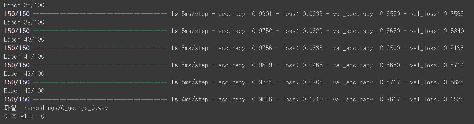
# 예측
for n in range(10):
  test_file = file_paths[100+n*300]
  print("파일:", test_file)
  print("예측 결과:", predict_digit(test_file))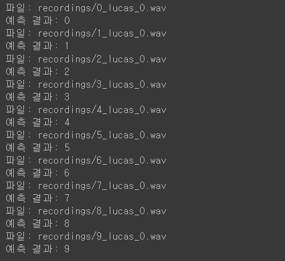
📌 Deeply Korean read speech corpus
# 1. 데이터 다운로드
!wget -O KoreanReadSpeechCorpus.tar.gz https://www.openslr.org/resources/97/KoreanReadSpeechCorpus.tar.gz

# 2. 압축 해제
!tar -xvzf KoreanReadSpeechCorpus.tar.gz
import json
import pandas as pd
# JSON 파일 로드
json_path = "/content/Korean_Read_Speech_Corpus_sample.json"
with open(json_path, "r", encoding="utf-8") as f:
data = json.load(f)
# 모든 발화의 (파일 경로, 텍스트) 추출
entries = []
for location, utterances in data.items():
for uid, info in utterances.items():
wav_path = f"/content/{location}/{uid}.wav"
text = info["text"]
entries.append({"wav_path": wav_path, "text": text})
# DataFrame 생성
df = pd.DataFrame(entries)
# 결과 확인
print(df.head())
from IPython.display import Audio, display

def play(index):
    if index < 0 or index >= len(df):
        print("잘못된 인덱스입니다.")
        return
    print(f"[{index}] 전사 문장:", df.iloc[index]["text"])
    display(Audio(df.iloc[index]["wav_path"], autoplay=False))
※ End-to-End 음성 인식 시스템 구현
# 1. 의존성 로드
import os, json, torch, librosa, hgtk
import numpy as np
import torch.nn as nn
from torch.utils.data import Dataset, DataLoader
from torch.nn.utils.rnn import pad_sequence
import torch.optim as optim

# 2. 자모 분리 함수
# 한글 문장을 받아서 모든 자모(초성,중성,종성) 단위로 분해
def split_jamos(text):
    result = []
    for ch in text:
        if hgtk.checker.is_hangul(ch):
            result.extend(hgtk.letter.decompose(ch))
        else:
            result.append(ch)
    return result

# 3. JSON 로드 및 samples 생성
with open("/content/Korean_Read_Speech_Corpus_sample.json", "r") as f:
    data = json.load(f)

samples = []
for fname, meta in data["AirbnbStudio"].items():
    path = f"/content/AirbnbStudio/{fname}.wav"
    if os.path.exists(path):
        samples.append({"path": path, "text": meta["text"]})

# 4. 자모 기반 vocab 구성
# 고유한 문자만 추출하여 사전 순으로 정렬
vocab = sorted(set(j for s in samples for j in split_jamos(s["text"])))
# 각 자모 문자에 고유한 인덱스를 부여하며, 인덱스-문자 간 양방향 매핑 생성
char2idx = {c: i + 1 for i, c in enumerate(vocab)}  # 0 = padding
idx2char = {i: c for c, i in char2idx.items()}
vocab_size = len(char2idx) + 1

# 5. Dataset 정의
class AttentionASRDataset(Dataset):
    def __init__(self, sample_list, max_len=300):
        self.samples = sample_list
        self.max_len = max_len

    def __len__(self):      # 데이터셋 길이 반환
        return len(self.samples)

    def __getitem__(self, idx):       # 지정한 idx에 해당하는 오디오 파일을 16kHz로 로드
        sample = self.samples[idx]
        y, sr = librosa.load(sample['path'], sr=16000)
        # MFCC를 추출하고 최대 길이로 잘라 텐서로 변환
        mfcc = librosa.feature.mfcc(y=y, sr=sr, n_mfcc=13).T
        if mfcc.shape[0] > self.max_len:
            mfcc = mfcc[:self.max_len]
        x = torch.tensor(mfcc, dtype=torch.float32)
		# 텍스트를 자모 분리하여 인덱스로 변환한 뒤 레이블 텐서로 반환
        jamos = split_jamos(sample['text'])
        label = [char2idx[c] for c in jamos]
        y = torch.tensor(label, dtype=torch.long)
        return x, y

# 6. Collate 함수 (패딩)
def collate_fn(batch):
    xs, ys = zip(*batch)     # 배치의 x와 y를 분리
    max_x = max([x.shape[0] for x in xs])     # 각 시퀀스의 최대 길이
    max_y = max([y.shape[0] for y in ys])
    # 시퀀스를 패딩하고 스택하여 배치 텐서를 생성
    padded_x = [torch.cat([x, torch.zeros(max_x - x.shape[0], x.shape[1])], dim=0) for x in xs]
    padded_y = [torch.cat([y, torch.zeros(max_y - y.shape[0], dtype=torch.long)], dim=0) for y in ys]
    return torch.stack(padded_x), torch.stack(padded_y)

# 7. 모델 정의
class Encoder(nn.Module):
	# 양방향 LSTM으로 정의된 인코더
    def __init__(self, input_dim, hidden_dim):
        super().__init__()
        self.lstm = nn.LSTM(input_dim, hidden_dim, batch_first=True, bidirectional=True)
	# 입력을 시퀀스 형태로 처리하여 출력
    def forward(self, x):
        output, _ = self.lstm(x)
        return output  # [B, T, 2H]


class AttentionDecoder(nn.Module):
    def __init__(self, hidden_dim, output_dim):
        super().__init__()
        self.embedding = nn.Embedding(output_dim, hidden_dim)    # 출력 토큰 임베딩
        # attention context와 embedding을 합쳐 LSTM에 넣고, 최종 예측을 위한 linear layer 구성
        self.lstm = nn.LSTM(hidden_dim + 2 * hidden_dim, hidden_dim, batch_first=True)
        self.attn = nn.Linear(hidden_dim + 2 * hidden_dim, 1)
        self.fc = nn.Linear(hidden_dim, output_dim)

    # 디코딩 시작: 인코더 출력과 target sequence 임베딩을 받아 준비
    def forward(self, enc_output, target_seq, max_len):
        B, T, H_enc = enc_output.shape  # H_enc = 256*2 = 512
        embedded = self.embedding(target_seq)  # [B, L, 256]
        outputs, hidden = [], None

        # 각 time step마다 decoder input + context를 attention으로 계산 -> LSTM -> Linear layer
        for t in range(max_len):
            query = embedded[:, t].unsqueeze(1).expand(-1, T, -1)  # [B, T, 256]
            attn_input = torch.cat([query, enc_output], dim=2)     # [B, T, 768]
            energy = self.attn(attn_input).squeeze(2)              # [B, T]
            attn_weights = torch.softmax(energy, dim=1).unsqueeze(1)  # [B, 1, T]
            context = torch.bmm(attn_weights, enc_output)          # [B, 1, 512]
            x = torch.cat([embedded[:, t:t+1, :], context], dim=2) # [B, 1, 768]
            out, hidden = self.lstm(x, hidden)                     # [B, 1, 256]
            output = self.fc(out.squeeze(1))                       # [B, vocab_size]
            outputs.append(output)

        return torch.stack(outputs, dim=1)  # [B, L, vocab_size]  모든 결과를 하나의 텐서로 반환

# 8. 학습 준비
train_set = AttentionASRDataset(samples)
train_loader = DataLoader(train_set, batch_size=8, shuffle=True, collate_fn=collate_fn)

device = torch.device("cuda" if torch.cuda.is_available() else "cpu")
encoder = Encoder(13, 256).to(device)
decoder = AttentionDecoder(256, vocab_size).to(device)

criterion = nn.CrossEntropyLoss(ignore_index=0)
optimizer = optim.Adam(list(encoder.parameters()) + list(decoder.parameters()), lr=1e-3)

# 9. 학습 루프
import matplotlib.pyplot as plt

# 학습 손실값 저장 리스트
loss_history = []

# 학습 루프 (충분한 학습 필요)
for epoch in range(100):
    encoder.train()
    decoder.train()
    total_loss = 0
    for x, y in train_loader:
        x, y = x.to(device), y.to(device)
        out_enc = encoder(x)  # [B, T, 512]
        out_dec = decoder(out_enc, y, max_len=y.size(1))  # [B, L, V]
        loss = criterion(out_dec.view(-1, vocab_size), y.view(-1))

        optimizer.zero_grad()
        loss.backward()
        optimizer.step()
        total_loss += loss.item()

    avg_loss = total_loss / len(train_loader)
    loss_history.append(avg_loss)
    print(f"Epoch {epoch+1}, Loss: {avg_loss:.4f}")

# 시각화
plt.figure(figsize=(8, 5))
plt.plot(loss_history, marker='o')
plt.title("Training Loss over Epochs")
plt.xlabel("Epoch")
plt.ylabel("Loss")
plt.grid(True)
plt.show()

# 모델 저장 디렉토리 설정
save_dir = "/content/asr_model"
os.makedirs(save_dir, exist_ok=True)

# 모델 저장
torch.save(encoder.state_dict(), os.path.join(save_dir, "encoder.pt"))
torch.save(decoder.state_dict(), os.path.join(save_dir, "decoder.pt"))

# 문자 집합 저장 (char2idx와 idx2char)
import pickle
with open(os.path.join(save_dir, "vocab.pkl"), "wb") as f:
    pickle.dump({
        "char2idx": char2idx,
        "idx2char": idx2char
    }, f)

print(f"모델과 문자 집합이 저장되었습니다: {save_dir}")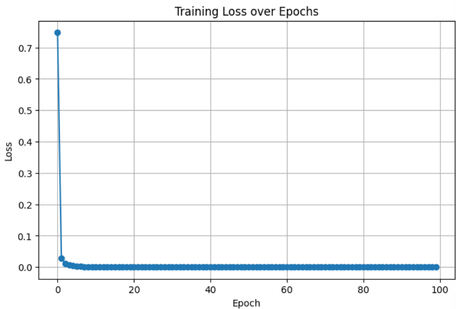
import hgtk

def greedy_decode(output_tensor):
    """ 디코더 출력 logits → 예측 문자 인덱스 → 자모 문자열 """
    pred_indices = output_tensor.argmax(2)  # [B, T]   # 각 step마다 확률이 가장 높은 자모 인덱스 선택
    pred_sequences = []      # 배치 안의 각 예측 시퀀스를 처리할 준비
    for seq in pred_indices:
        result = []
        for idx in seq:
            if idx.item() != 0:  # padding 제외
                result.append(idx2char.get(idx.item(), ""))    # 자모 문자로 변환
        pred_sequences.append(result)
    return pred_sequences

# 자모 시퀀스를 완전한 음절 단위로 조합
def merge_jamos(jamo_seq):
    result = ""
    i = 0
    while i < len(jamo_seq):
        try:
            cho = jamo_seq[i]
            jung = jamo_seq[i + 1]
            if i + 2 < len(jamo_seq):
                jong = jamo_seq[i + 2]
                try:
                    result += hgtk.letter.compose(cho, jung, jong)
                    i += 3
                except hgtk.exception.NotHangulException:
                    result += hgtk.letter.compose(cho, jung)
                    i += 2
            else:
                result += hgtk.letter.compose(cho, jung)
                i += 2
        except:
            result += ''.join(jamo_seq[i:])
            break
    return result
# 하나의 .wav 파일을 입력받아 음성 결과를 출력하는 함수
def infer(file_path):
# 1) 음성 로드 및 MFCC 추출
y, sr = librosa.load(file_path, sr=16000)
# MFCC를 추출하고 전치
mfcc = librosa.feature.mfcc(y=y, sr=sr, n_mfcc=13).T
mfcc_tensor = torch.tensor(mfcc[:300], dtype=torch.float32).unsqueeze(0).to(device) # [1, T, 13]
# 2) 모델 추론
encoder.eval()
decoder.eval()
with torch.no_grad():
enc_output = encoder(mfcc_tensor) # 인코더를 통해 음성 시퀀스를 입베딩 및 벡터로 변환
dummy_target = torch.zeros((1, 30), dtype=torch.long).to(device) # 최대 추론 길이만큼 빈 타겟
output = decoder(enc_output, dummy_target, max_len=30)
# 3) 디코딩
jamo_seq = greedy_decode(output)[0]
result = merge_jamos(jamo_seq)
print("자모:", "".join(jamo_seq))
print("결과:", result)
return result# AirbnbStudio의 파일 중 하나
infer("/content/AirbnbStudio/sub100100a00000.wav")
728x90
'음성처리' 카테고리의 다른 글
| [음성 인식]ASR 모델 평가(WER, CER, Accuracy) (0) | 2025.07.25 |
|---|---|
| [음성 인식]최신 ASR 모델(CTC, Transformer, Conformer, Self-Supervised Learning, Whisper) (0) | 2025.07.24 |
| [음성 인식]CTC 기반 ASR (1) | 2025.07.21 |
| [딥러닝]TensorFlow/PyTorch 기반 ASR 모델 (0) | 2025.07.19 |
| [딥러닝]ASR 시스템, CTC, Transformer (0) | 2025.07.19 |


